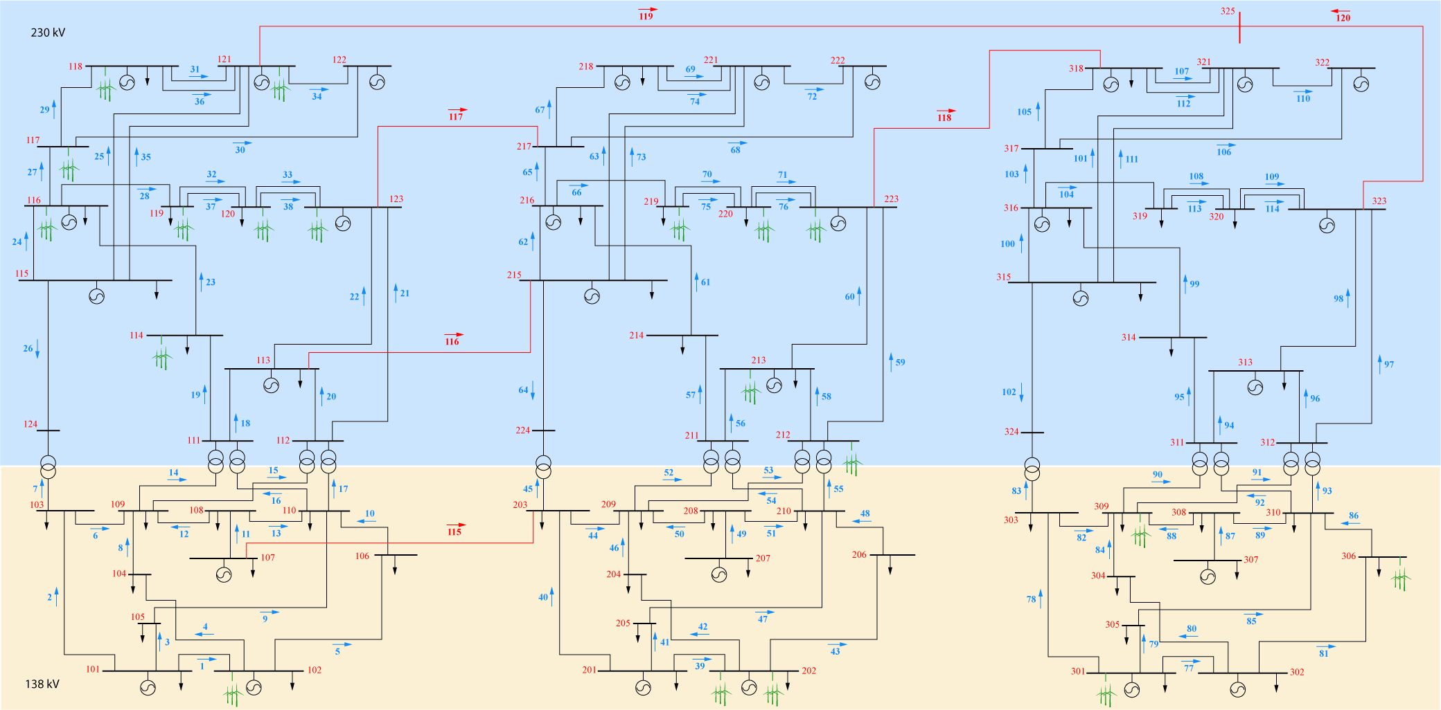
We will now move from the three bus example to the IEEE RTS. You can find a brief description of this system below or visit this link for details.
The IEEE RTS system includes 96 generators distributed among 73 buses and connected by 120 lines. The specific characteristics of generators can be found here.
We also added 19 wind farms to the IEEE RTS system, which are characterized as follows:
In [ ]:


using MAT # This package enables reading .mat files
using JuMP
using Gadfly
using Interact
For the following experiments we prepare the input file (ieee_test_system.mat) with all input data needed. In the following simulations we demonstrate how these inputs can be imported directly to Julia.
In [ ]:


file = matopen("ieee_test_system.mat") # open the .mat file with input data
c_g=read(file, "c_g") # incremental costs of generators
c_g0=read(file, "c_g0") # no load costs of generators
g_max=read(file, "g_max") # maximum power outputs of generators
g_min=read(file, "g_min") # minimum power outputs of generators
g_map=read(file, "g_map") # map of generators

d=read(file, "d") # demand

w_f=read(file, "w_f") # wind forecasts for each wind farm
w_map=read(file, "w_map") # map of wind farms

f_map=read(file, "f_map") # map of transmission lines
f_max=read(file, "f_max") #maximum power flow limits of transmission lines
x=read(file, "x") # reactance of transmission lines
close(file)

N_gen = length (c_g) # number of generators
N_bus = length(d) # number of buses
N_line = length (f_max) # number of lines
N_wind = length (w_f) # number of wind farms


c_w = 10 # dispatch cost of wind generation
The following cell displays the economic dispatch model:
In [ ]:


function solve_ed (g_max, g_min, c_g, c_w, d, w_f)
#Define the economic dispatch (ED) model
ed=Model()

# Define decision variables
    @defVar(ed, 0 <= g[i=1:N_gen] <= g_max[i]) # power output of generators
@defVar(ed, 0 <= w  <= w_f ) # wind power injection

# Define the objective function
    @setObjective(ed,Min,sum{c_g[i] * g[i],i=1:N_gen}+ c_w * w)

# Define the constraint on the maximum and minimum power output of each generator
    for i in 1:N_gen
    @addConstraint(ed,  g[i] <= g_max[i]) #maximum
    @addConstraint(ed,  g[i] >= g_min[i]) #minimum
end


# Define the constraint on the wind power injection
@addConstraint(ed, w <= w_f)

# Define the power balance constraint
    @addConstraint(ed, sum{g[i],i=1:N_gen} + w == d)

# Solve statement
solve(ed)
    # return the optimal value of the objective function and its minimizers
    return getValue(g)[:], getValue(w), w_f-getValue(w), getObjectiveValue(ed)
end
We use the IEEE RTS system to observe the impact of demand on the total cost and dispatch of individual generators. It can also be observed that different wind generation conditions affect dispatch of generators, even for a fixed demand value.
In [ ]:


@manipulate for d = sum(g_min):1:sum(g_max)
    g_opt,w_opt,ws_opt,obj = solve_ed (g_max, g_min, c_g, c_w, sum(d), sum(w_f))

   html("Total cost, \$: $obj")
end
In [ ]:


@manipulate for d = sum(g_min):1:sum(g_max), w_scale = 0.5:0.01:1.5
    g_opt,w_opt,ws_opt,obj = solve_ed (g_max, g_min, c_g, c_w, sum(d), w_scale*sum(w_f))

    set_default_plot_size(16cm, 10cm)

    # Plot dispatch of every generator
    plot(x=1:1:N_gen,y=[g_opt], Geom.bar,
    Guide.XLabel("Index of generators "), Guide.YLabel("Dispatch, MW"))
end
In the following cell we duplicate the UC model presented earlier.
In [ ]:


function solve_uc (g_max, g_min, c_g, c_w, d, w_f)
#Define the unit commitment (UC) model

uc=Model()

# Define decision variables
    @defVar(uc, 0 <= g[i=1:N_gen] <= g_max[i]) # power output of generators
    @defVar(uc, u[i=1:N_gen], Bin) # Binary status of generators
@defVar(uc, 0 <= w  <= w_f ) # wind power injection

# Define the objective function
    @setObjective(uc,Min,sum{c_g[i] * g[i],i=1:N_gen}+ c_w * w)

# Define the constraint on the maximum and minimum power output of each generator
for i in 1:N_gen
    @addConstraint(uc,  g[i] <= g_max[i] * u[i]) #maximum
    @addConstraint(uc,  g[i] >= g_min[i] * u[i]) #minimum
end


# Define the constraint on the wind power injection
@addConstraint(uc, w <= w_f)

# Define the power balance constraint
    @addConstraint(uc, sum{g[i], i=1:N_gen} + w == d)

# Solve statement
    status = solve(uc)

    return status, getValue(g)[:], getValue(w), w_f-getValue(w), getValue(u)[:], getObjectiveValue(uc)
end
We can now use the manipulator to gradually adjust the demand and observe its impact on the total cost. Note that the UC model results in a more cost-effective solution than the ED model.
In [ ]:


@manipulate for d = sum(g_min):1:sum(g_max)
    status,g_opt,w_opt,ws_opt,u_opt,obj = solve_uc (g_max, g_min, c_g, c_w, sum(d), sum(w_f));

   html("Total cost, \$: $obj")
end
In this experiment, we will adjust the value of demand and wind power forecast to observe their impacts on the commitment and dispatch decisions of generators. Note that these decisions are drastically different from the economic dispatch decisions.
In [ ]:


@manipulate for d = sum(g_min):1:sum(g_max), w_scale = 0.5:0.01:1.5
    status,g_opt,w_opt,ws_opt,u_opt,obj = solve_uc (g_max, g_min, c_g, c_w, sum(d), w_scale*sum(w_f));

    set_default_plot_size(16cm, 20cm)
    # Plot dispatch of every generator
    vstack(plot(x=1:1:N_gen,y=[g_opt], Geom.bar,
    Guide.XLabel("Index of generators "), Guide.YLabel("Dispatch, MW")),
    plot(x=1:1:N_gen,y=[u_opt], Geom.bar,
    Guide.XLabel("Index of generators "), Guide.YLabel("Commitment status")))

end
In the following cell we present the code for the OPF model:
In [ ]:


function solve_dcopf (g_max, g_min, c_g, c_w, d, w_f, g_map, f_map, w_map, f_max, x)
#Define the optimal power flow (OPF) model

opf=Model()

# Define decision variables
@defVar(opf,   g[i=1:N_gen] >= 0 ) ; # power output of generators
@defVar(opf, w[v=1:N_wind] >=0 ) ; # wind power injection
@defVar(opf, f[l=1:N_line]) ; # power flows
@defVar(opf, theta[b=1:N_bus]) ; # bus angle


# Define the objective function
@setObjective(opf,Min,sum{c_g[i] * g[i],i=1:N_gen} + sum{c_w * w[v],v=1:N_wind});


for i in 1:N_gen
        @addConstraint(opf,  g[i] <= g_max[i]  ) #maximum
        @addConstraint(opf,  g[i] >= g_min[i]  ) #minimum
end


# Define the constraint on the wind power injections
for v in 1:N_wind
    @addConstraint(opf,  w[v] <= w_f[v]);
end

# Define the constraint on the power flows
for l in 1:N_line
    @addConstraint(opf, f[l] <= f_max[l]); # direct flows
    @addConstraint(opf, f[l] >=  -f_max[l]); # reverse flows
end

# Define the power balance constraint
for b in 1:N_bus
        @addConstraint(opf, sum{g_map[i,b]* g[i],i=1:N_gen}  + sum{w_map[v,b] * w[v], v=1:N_wind}  + sum{f_map[l,b] * f[l], l=1:N_line}>= d[b]);
end

# Calculate f[l]
for l in 1:N_line
    @addConstraint(opf, x[l] * f[l] ==  sum{f_map [l,b] * theta[b], b=1:N_bus})  ; # power flow in every line
end

# Slack bus
    @addConstraint(opf, theta [b=1] == 0)  ; # set the slack bus


# Solve statement
status = solve(opf)

    return status, getObjectiveValue(opf), getValue(g)[:], getValue(f)[:], getValue(w)[:]
end
In the next experiment we use three manipulators, adjusting the power flow limits on transmission lines, demand and wind power generation, to observe their impact on the total cost.
In [ ]:


@manipulate for f_scale = 0.4 : 0.01 : 1.0, d_scale = 0.5:0.01:1.5, w_scale = 0.5:0.01:1.0


    status, obj, g_opt, f_opt, w_opt = solve_dcopf(g_max, g_min, c_g, c_w, d_scale*d, w_scale*w_f, g_map, f_map, w_map, f_scale*f_max, x)

    html("Total cost, \$: $obj")

end
Again, we use three manipulators, adjusting the power flow limits on transmission lines, demand and wind power generation, to observe their impact on the the power flows of transmission lines, dispatch decisions of generators and wind power generation.
In [ ]:


@manipulate for f_scale = 0.4 : 0.01 : 1.0, d_scale = 0.5:0.01:1.5, w_scale = 0.5:0.01:1.0
    status, obj, g_opt, f_opt, w_opt = solve_dcopf(g_max, g_min, c_g, c_w, d_scale*d, w_scale*w_f, g_map, f_map, w_map, f_scale*f_max, x)

    set_default_plot_size(16cm, 30cm)
    # Plot dispatch of every generator
    vstack(plot(x=1:N_line,y=[abs(f_opt)], Geom.bar,
    Guide.XLabel("Index of lines "), Guide.YLabel("Flow, MW")),
    plot(x=1:N_gen,y=[g_opt], Geom.bar,
    Guide.XLabel("Index of generators "), Guide.YLabel("Dispatch of generators, MW")),
    plot(x=1:N_wind,y=[w_opt], Geom.bar,
    Guide.XLabel("Index of wind farms "), Guide.YLabel("Dispatch of wind, MW"))
    )


end
In this section we will show how the power flows can be graphically represented in an interactive fashion.
In [ ]:


using GraphViz # package used for drawing graphs

function writeDot(name, busIdx, busInj, renGen, f, t, lineFlow, lineLim, size=(11,14))
    # This function generates a graph that richly expresses the RTS96 system state.
    # name              a name for the graph and resulting dot file
    # busIdx            bus names (could be text) in order of busInj
    # busInj            injection at each bus
    # renGen            renewable generation at each bus (0 for non-wind buses)
    # f                 "from" node for each line
    # t                 "to" node for each line
    # lineFlow          flow on each line
    # lineLim           limit for each line
    # size              size of graphical output

    busInj = round(busInj,2)
    lineFlow = round(lineFlow,2)

    # Open the dot file, overwriting anything already there:
    dotfile = IOBuffer()

    # Begin writing the dot file:
    write(dotfile, "digraph $(name) {\nrankdir=LR;\n")

    # Set graph properties:
    write(dotfile,
    "graph [fontname=helvetica, tooltip=\" \", overlap=false, size=\"$(size[1]),$(size[2])\", ratio=fill, orientation=\"portrait\",layout=dot];\n")

    # Set default node properties:
    write(dotfile, "node [fontname=helvetica, shape=square, style=filled, fontsize=20, color=\"#bdbdbd\"];\n")

    # Set default edge properties:
    write(dotfile, "edge [fontname=helvetica, style=\"setlinewidth(5)\"];\n")

    # Write bus data to dot file:
    for i = 1:length(busIdx)
        write(dotfile,
        "$(i) [label=$(int(busIdx[i])), tooltip=\"Inj = $(busInj[i])\"") # bus label and tooltip

        # Represent renewable nodes with blue circles:
        if union(find(renGen),i) == find(renGen)
            write(dotfile, ", shape=circle, color=\"#5677fc\"")
        end

        write(dotfile, "];\n")
    end

    # Write line data to file:

    for i = 1:length(f)

        normStrain = abs(lineFlow[i])/lineLim[i] # normalized strain on line i

        # Use flow direction to determine arrow direction,
        # label with flow,
        # and color according to strain
        #if lineFlow[i] > 0
            write(dotfile,
            "$(f[i]) -> $(t[i]) [label=$(lineFlow[i])")
        #else
        #    write(dotfile,
        #    "$(t[i]) -> $(f[i]) [label=$(-lineFlow[i])")
        #end
        write(dotfile,
        ", tooltip=\" \", labeltooltip=\"Flow = $(int(normStrain*100))%\", color=\"$(abs(round((1 - normStrain)/3,3))) 1.000 0.700\"];\n")
    end

    write(dotfile, "}\n")

    dottext = takebuf_string(dotfile)
    #print(dottext)

    return Graph(dottext)
end
In [ ]:


# We need to reformat the input data
from_node = [find(f_map[i,:] .== 1)[1] for i in 1:size(f_map,1)];
to_node = [find(f_map[i,:] .== -1)[1] for i in 1:size(f_map,1)];


@manipulate for f_scale = 0.4 : 0.01 : 1.0
    status, obj, g_opt, f_opt, w_opt = solve_dcopf(g_max, g_min, c_g, c_w, d, w_f, g_map, f_map, w_map, f_scale*f_max, x)

    wind_bus = zeros(N_bus)
    for i in 1:N_wind
        wind_idx = find(w_map[i,:] .== 1)[1]
        wind_bus[wind_idx] = f_opt[i]
    end


    writeDot("OPF", [i for i in 1:N_bus], g_opt, wind_bus, from_node, to_node, f_opt, f_scale*f_max, (8,8))

end
After discussing the ED, UC, and OPF models and testing them on the IEEE RTS system, we believe you can try to implement thee following simple model:
In [ ]: